Growth of Functions in Design and Analysis of Algorithms (DAA)

---

❮ Previous    Next ❯

---

---

Objective

The objectives of studying Growth of Functions are:

• Understand how algorithm running time changes with input size.
• Compare two or more algorithms mathematically.
• Identify efficient algorithms for solving computational problems.
• Understand the concept of scalability.
• Prepare for the study of Big-O, Big-Ω and Big-Θ notations.

---

Introduction

Suppose we have two sorting algorithms. Algorithm A takes

• 100 operations for 10 elements
• 1,000 operations for 100 elements
• 10,000 operations for 1,000 elements

Algorithm B takes

• 100 operations for 10 elements
• 10,000 operations for 100 elements
• 1,000,000 operations for 1,000 elements

Both algorithms work correctly, but Algorithm A grows much slower than Algorithm B. Therefore, Algorithm A is considered more efficient for large inputs. This increase in running time with respect to input size is known as the Growth of Function.

---

Definition of Growth of Functions

Growth of Functions describes how the running time or memory requirement of an algorithm increases as the size of input (n) increases. Instead of calculating the exact running time, we analyze the mathematical function that represents the number of operations performed.

T(n) = Number of Operations performed by an Algorithm

Where,

• T(n) = Running time
• n = Input size

---

Why Do We Study Growth of Functions?

Reason	Explanation
Hardware Independent	Performance comparison does not depend on computer speed.
Language Independent	Works for algorithms written in any programming language.
Predict Future Performance	Estimates running time for very large inputs.
Select Better Algorithm	Helps choose the most efficient algorithm.
Optimization	Improves software performance.

---

Input Size (n)

The efficiency of an algorithm mainly depends upon the size of the input. Examples:

Problem	Input Size
Searching an Array	Number of elements
Sorting	Total records
Graph Algorithms	Vertices and Edges
Matrix Multiplication	Order of Matrix
String Matching	Length of String

---

Running Time Function

Every algorithm can be represented by a mathematical function. Examples:

Algorithm	Running Time
Finding Maximum Element	T(n)=n
Binary Search	T(n)=log n
Merge Sort	T(n)=n log n
Bubble Sort (Worst Case)	T(n)=n²
Tower of Hanoi	T(n)=2ⁿ

---

Example of Growth

Suppose an algorithm performs:

T(n)=5n²+7n+20

When n becomes very large, the term 5n² dominates the remaining terms. Therefore,

T(n)=O(n²)

The constants (5, 7 and 20) become insignificant for large input sizes. Only the fastest growing term is considered while analyzing algorithms.

---

Graphical Representation of Growth of Functions

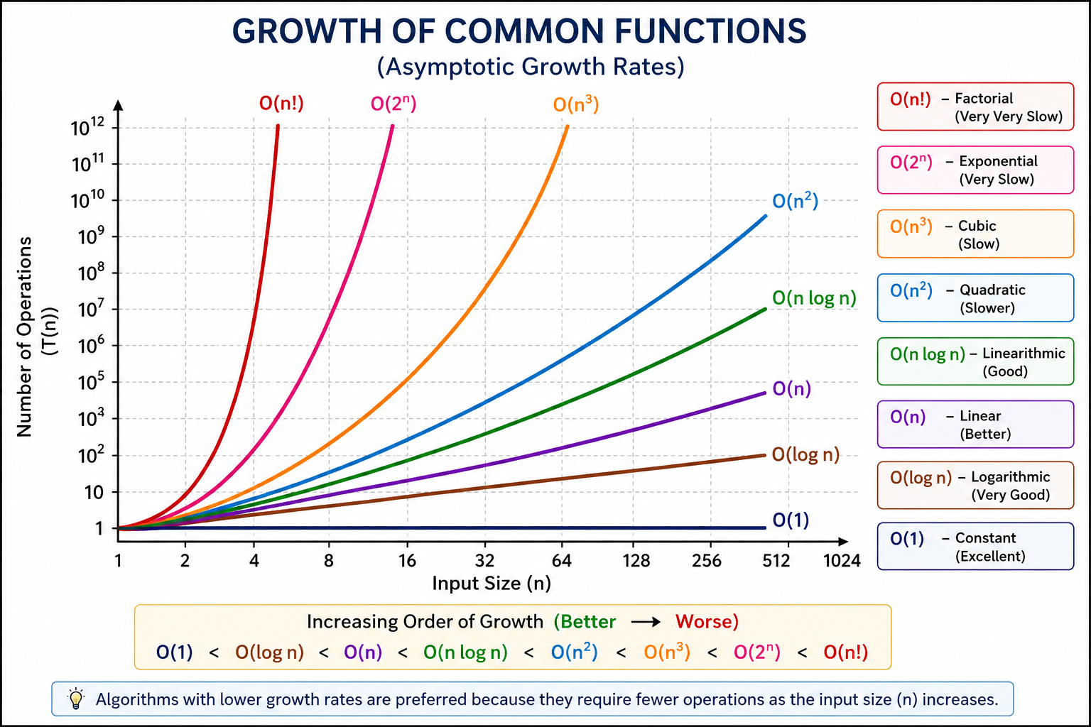
The following graph compares the growth of commonly used mathematical functions.

---

Order of Growth

The order of growth tells us how rapidly the running time of an algorithm increases with increasing input size. Algorithms having lower order of growth are considered more efficient.

---

Common Growth Functions

Growth Function	Name	Efficiency
1	Constant	Excellent
log n	Logarithmic	Very Fast
n	Linear	Good
n log n	Linearithmic	Efficient
n²	Quadratic	Slow
n³	Cubic	Very Slow
2ⁿ	Exponential	Extremely Slow
n!	Factorial	Worst Practical Growth

---

Types of Growth of Functions

The running time of an algorithm can grow in different ways depending on the number of operations it performs. The following are the most commonly used growth functions in Design and Analysis of Algorithms.

---

1. Constant Growth – O(1)

An algorithm is said to have Constant Time Complexity if the number of operations remains the same irrespective of the input size. Whether there is one element or one million elements, the execution time remains almost constant.

T(n) = c

Example

Accessing the first element of an array.

int first = arr[0];

Input Size (n)	Operations
10	1
100	1
1000	1
1000000	1

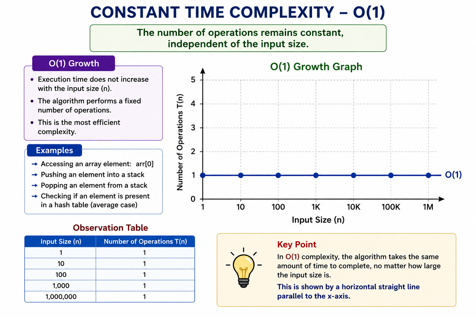
Image Required: A horizontal straight line representing constant growth.

---

2. Logarithmic Growth – O(log n)

In logarithmic growth, the problem size reduces after every iteration. Instead of processing all elements, the algorithm repeatedly divides the problem into two equal halves. This makes logarithmic algorithms extremely efficient for large inputs.

T(n)=log n

Example

• Binary Search
• Searching in Balanced Binary Search Tree
• AVL Tree Search

Input Size	Maximum Comparisons
16	4
32	5
64	6
1024	10

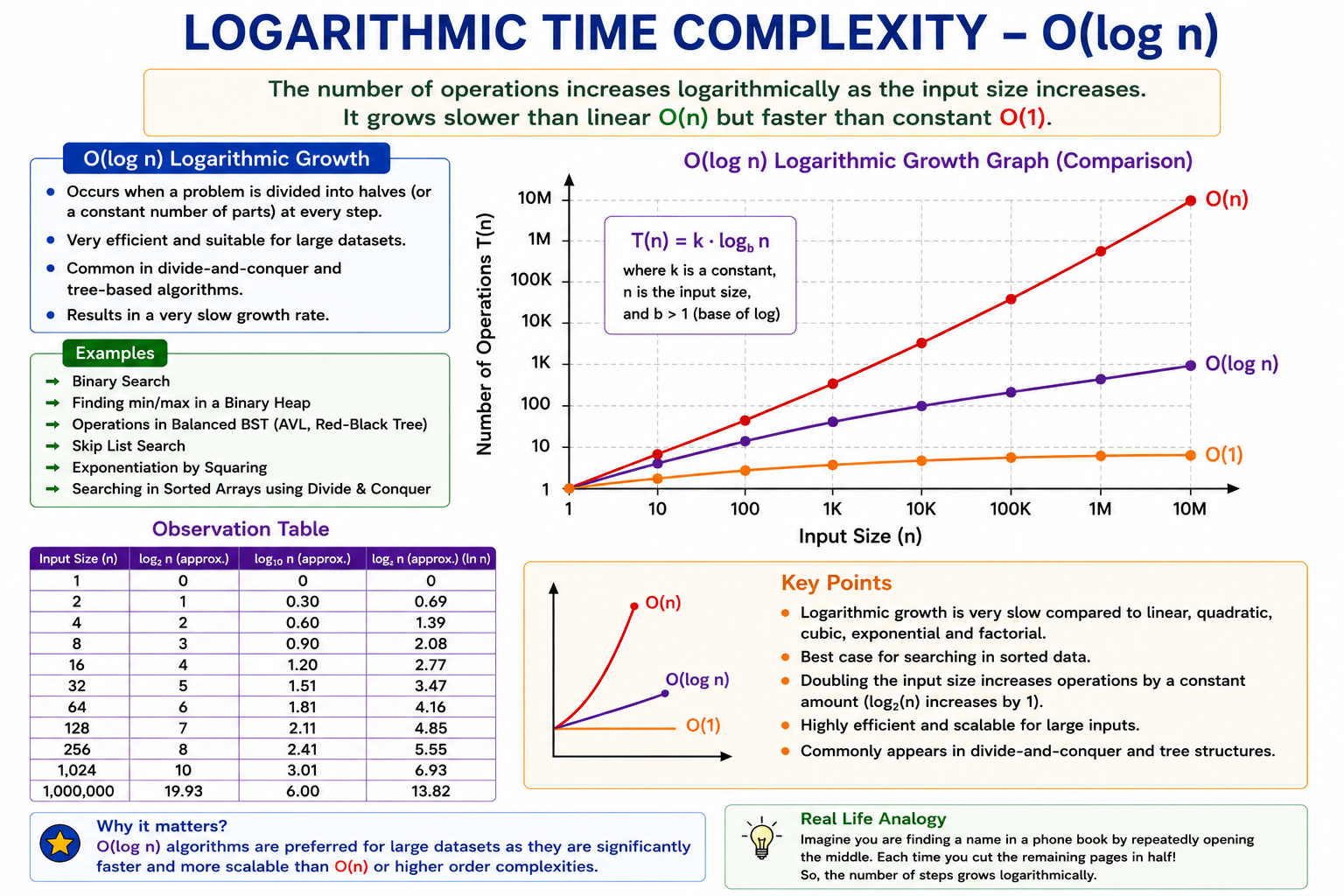
Image Required: A slowly increasing logarithmic curve.

---

3. Linear Growth – O(n)

In linear growth, the running time increases directly proportional to the input size. If the input doubles, the running time approximately doubles.

T(n)=n

Examples

• Linear Search
• Finding Maximum Element
• Traversing an Array

Input Size	Operations
10	10
100	100
1000	1000
10000	10000

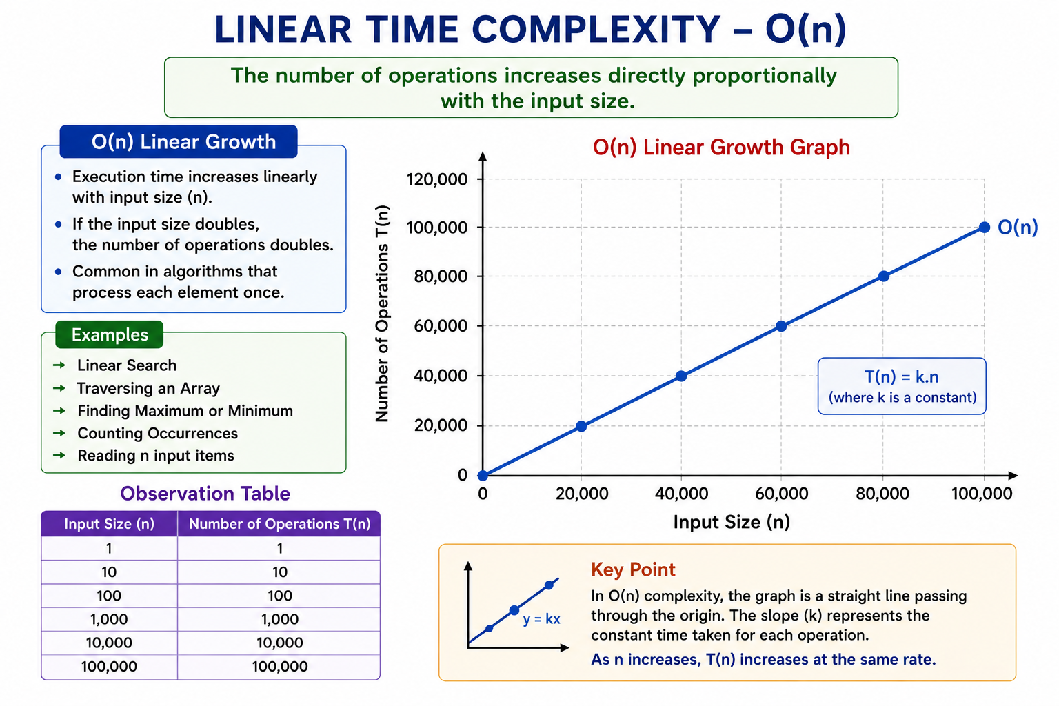
Image Required: Straight diagonal line showing linear growth.

---

4. Linearithmic Growth – O(n log n)

Linearithmic growth is obtained when an algorithm divides the problem and then processes all elements. This complexity is considered highly efficient for sorting algorithms.

Examples

• Merge Sort
• Heap Sort
• Efficient Quick Sort (Average Case)

Input Size	Approximate Operations
100	664
1000	9965
10000	132877

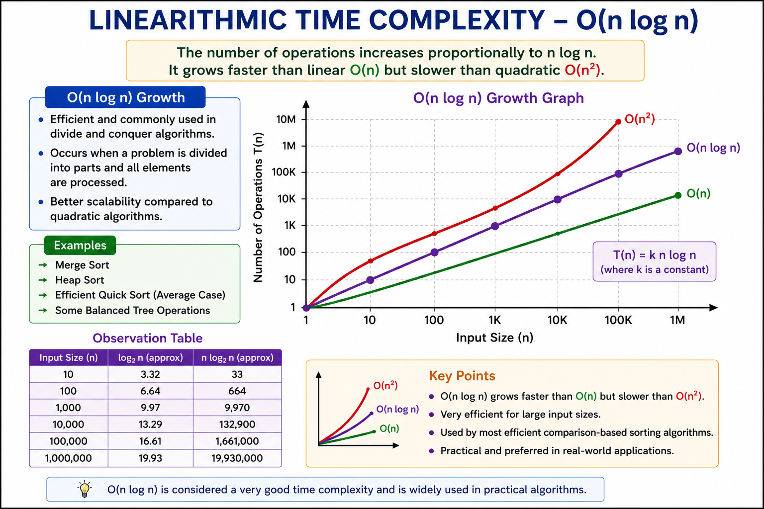
Image Required: Curve lying between Linear and Quadratic growth.

---

5. Quadratic Growth – O(n²)

Quadratic growth occurs when every element is compared with every other element. Usually generated by two nested loops.

T(n)=n²

Examples

• Bubble Sort
• Selection Sort
• Insertion Sort (Worst Case)

for(i=0;i<n;i++)
{
    for(j=0;j<n;j++)
    {
        // Operation
    }
}

Input Size	Operations
10	100
100	10000
1000	1000000

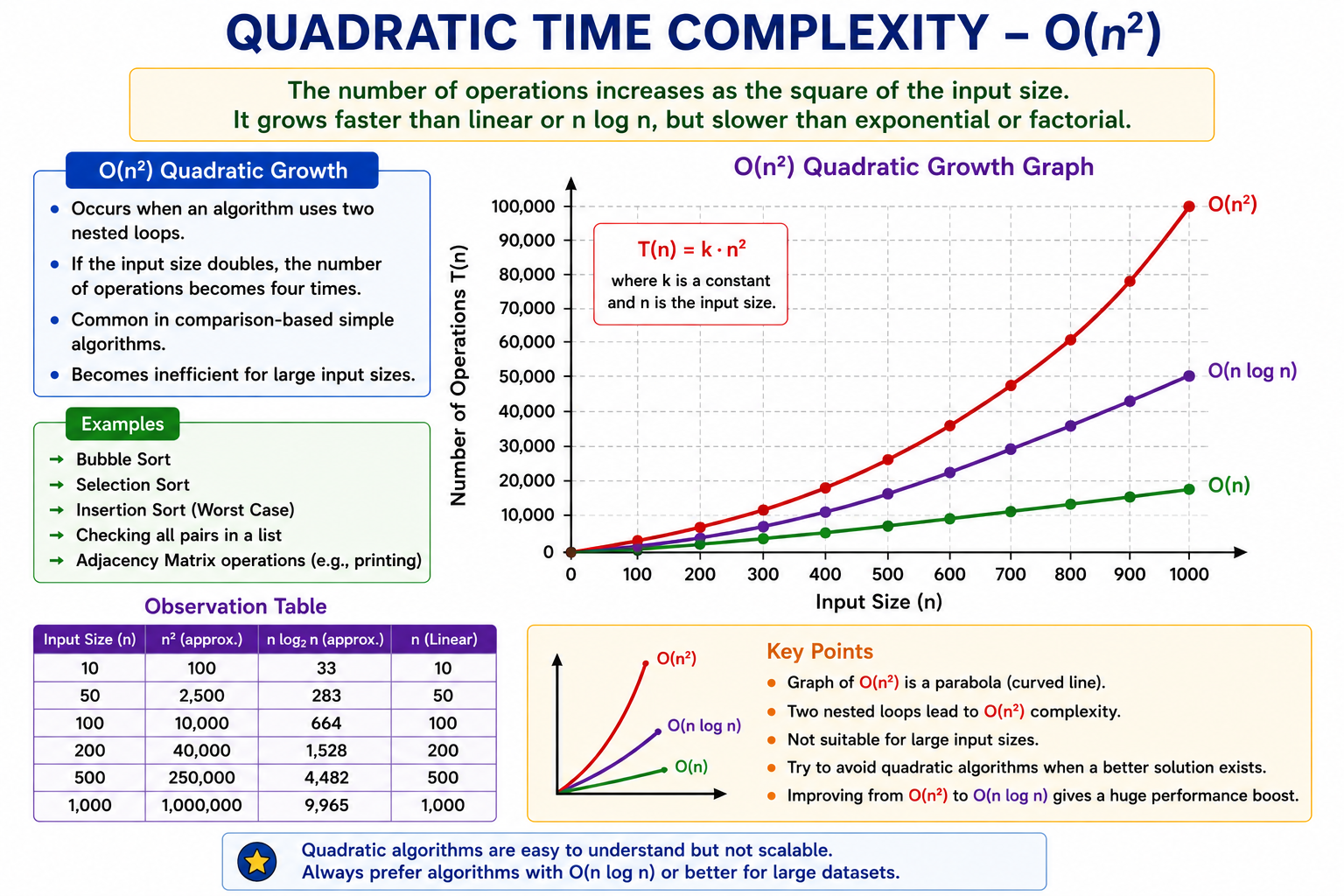
Image Required: Parabolic curve representing O(n²).

---

6. Cubic Growth – O(n³)

Cubic complexity occurs when three nested loops execute. These algorithms become very slow for large values of n.

for(i=0;i<n;i++)
{
    for(j=0;j<n;j++)
    {
        for(k=0;k<n;k++)
        {

        }
    }
}

Examples

• Basic Matrix Multiplication
• Some Dynamic Programming Problems
• 3-Dimensional Array Processing

Input Size	Operations
10	1000
100	1000000
1000	1000000000

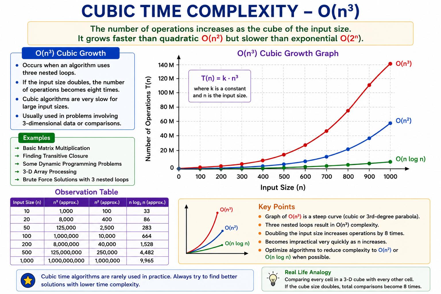
Image Required: Steep cubic curve increasing faster than O(n²).

---

7. Exponential Growth – O(2ⁿ)

An algorithm exhibits Exponential Growth when the number of operations doubles with every increase in the input size. Such algorithms become impractical even for moderately large values of n because the running time increases very rapidly.

T(n) = 2ⁿ

Examples

• Recursive Fibonacci Algorithm (without Dynamic Programming)
• Tower of Hanoi
• Generating All Possible Subsets
• Backtracking Problems (Worst Case)

Input Size (n)	Operations (2n)
5	32
10	1,024
20	1,048,576
30	1,073,741,824

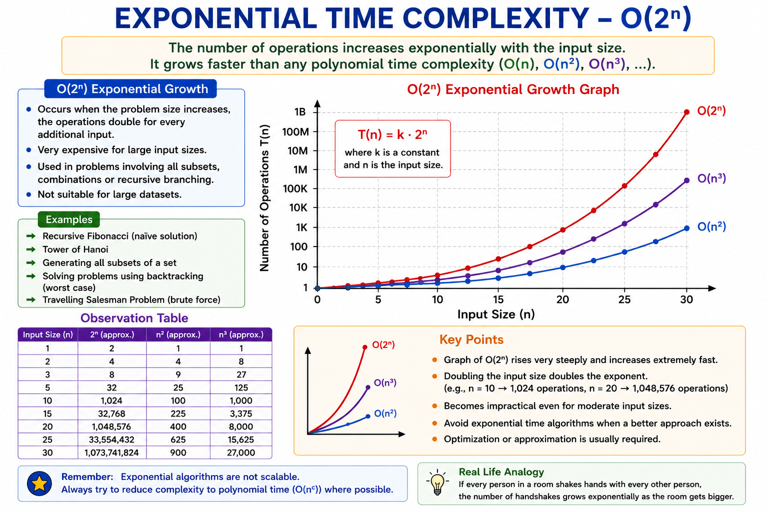
Image Required: A rapidly rising exponential curve showing O(2ⁿ).

---

8. Factorial Growth – O(n!)

Factorial Growth is one of the slowest practical growth rates. It occurs when an algorithm generates every possible arrangement (permutation) of the input. Since the number of permutations grows extremely fast, factorial algorithms become impractical even for small values of n.

T(n)=n!

Examples

• Travelling Salesman Problem (Brute Force)
• Generating All Permutations
• Brute Force Scheduling Algorithms

n	n!
3	6
5	120
8	40,320
10	3,628,800
15	1,307,674,368,000

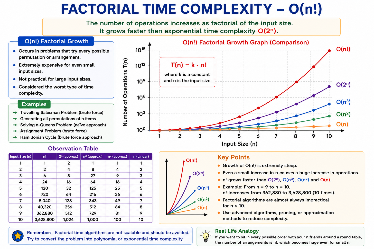
Image Required: A curve increasing even faster than O(2ⁿ).

---

Comparison of Common Growth Functions

The following table compares the most commonly encountered growth functions in algorithm analysis.

Growth Function	Name	Efficiency	Example Algorithm
O(1)	Constant	Excellent	Array Index Access
O(log n)	Logarithmic	Very Fast	Binary Search
O(n)	Linear	Good	Linear Search
O(n log n)	Linearithmic	Efficient	Merge Sort
O(n²)	Quadratic	Slow	Bubble Sort
O(n³)	Cubic	Very Slow	Basic Matrix Multiplication
O(2n)	Exponential	Extremely Slow	Recursive Fibonacci
O(n!)	Factorial	Worst Practical	Travelling Salesman (Brute Force)

---

Ranking of Growth Functions

The efficiency of algorithms decreases as the growth function increases.

O(1) < O(log n) < O(n) < O(n log n) < O(n²) < O(n³) < O(2ⁿ) < O(n!)

---

Growth Comparison for Different Input Sizes

n	O(1)	O(log n)	O(n)	O(n log n)	O(n²)	O(2n)
10	1	3	10	33	100	1024
100	1	7	100	664	10000	Very Large
1000	1	10	1000	9965	1000000	Impossible to Compute

---

Real-Life Examples of Growth Functions

Growth	Real-Life Example
O(1)	Switching on a light bulb.
O(log n)	Finding a word in a dictionary.
O(n)	Checking every student in a classroom.
O(n log n)	Sorting examination records using Merge Sort.
O(n²)	Comparing every student with every other student.
O(n³)	Processing every cell of a three-dimensional cube.
O(2n)	Trying every possible binary combination.
O(n!)	Trying every possible seating arrangement of people.

---

Importance of Growth of Functions in DAA

• Helps compare algorithms mathematically.
• Predicts performance for very large input sizes.
• Removes hardware dependency from analysis.
• Forms the basis of Asymptotic Analysis.
• Helps software engineers design efficient applications.
• Reduces execution time and resource consumption.
• Improves scalability of software systems.

---

---

Common Mistakes Made by Students

• Comparing actual execution time instead of growth rate.
• Ignoring the dominant term while finding complexity.
• Considering constants in asymptotic analysis.
• Confusing O(n log n) with O(log n).
• Assuming recursive algorithms are always slow.
• Using Bubble Sort for very large datasets.

---

Solved Numerical Examples

The following examples illustrate how to determine the order of growth of different mathematical functions.

---

Example 1

Find the order of growth of

T(n) = 7n² + 12n + 25

Solution:

• The highest degree term is 7n².
• For very large values of n, the terms 12n and 25 become insignificant.
• Ignore constants and lower-order terms.

Therefore, T(n) = O(n²)

---

Example 2

Find the order of growth of

T(n)=50n log n + 100n

Solution:

Since n log n grows faster than n, the dominant term is n log n.

T(n)=O(n log n)

---

Example 3

Find the order of growth of

T(n)=1000 + 25

The function does not depend upon the input size.

T(n)=O(1)

---

Quick Revision Table

Complexity	Name	Example
O(1)	Constant	Array Access
O(log n)	Logarithmic	Binary Search
O(n)	Linear	Linear Search
O(n log n)	Linearithmic	Merge Sort
O(n²)	Quadratic	Bubble Sort
O(n³)	Cubic	Matrix Multiplication
O(2n)	Exponential	Tower of Hanoi
O(n!)	Factorial	Travelling Salesman (Brute Force)

---

Applications of Growth of Functions

• Designing efficient algorithms.
• Performance comparison of algorithms.
• Selection of appropriate data structures.
• Compiler optimization.
• Artificial Intelligence algorithms.
• Machine Learning applications.
• Database query optimization.
• Computer Graphics.
• Network routing algorithms.
• Operating System scheduling.

---

Advantages

• Provides hardware-independent performance analysis.
• Helps compare different algorithms fairly.
• Predicts performance for very large inputs.
• Simplifies mathematical analysis.
• Assists in selecting scalable algorithms.
• Reduces software execution time.

---

Limitations

• Ignores constant execution time.
• Does not consider compiler optimization.
• Does not include hardware characteristics.
• Small input performance may differ from theoretical analysis.

---

Difference Between Actual Running Time and Growth of Function

Actual Running Time	Growth of Function
Depends on hardware.	Independent of hardware.
Depends on compiler.	Independent of compiler.
Measured in seconds.	Measured mathematically.
Changes with processor speed.	Depends only on input size.
Useful for benchmarking.	Useful for algorithm analysis.

---

---

AKTU Previous Year Examination Questions

1. Define Growth of Functions with suitable examples.
2. Explain the need for Growth of Functions in algorithm analysis.
3. Compare O(n), O(n²) and O(n log n).
4. Arrange the common growth functions in increasing order.
5. Explain exponential and factorial growth with examples.
6. Why are lower-order terms ignored during asymptotic analysis?
7. Discuss the importance of Growth of Functions in DAA.

---

Frequently Asked Viva Questions

1. What is Growth of Functions?
2. Why do we ignore constants during complexity analysis?
3. Which growth function is the fastest?
4. Which growth function is the slowest?
5. What is meant by dominant term?
6. Which sorting algorithm has O(n log n) complexity?
7. Why is Binary Search faster than Linear Search?
8. What is scalability?
9. What is input size?
10. Why is algorithm analysis important?

---

Frequently Asked Interview Questions

1. Explain Growth of Functions using real-life examples.
2. Differentiate O(n) and O(log n).
3. Which complexity is better: O(n log n) or O(n²)? Why?
4. Why is Bubble Sort inefficient for large datasets?
5. Can an algorithm have multiple complexity expressions?
6. What is the importance of dominant terms?
7. Why do exponential algorithms perform poorly?
8. How do growth functions help software engineers?

---

Practice Questions

1. Find the order of growth of T(n)=6n²+3n+5.
2. Find the order of growth of T(n)=15n log n + n.
3. Arrange O(1), O(n²), O(log n), O(n log n) in increasing order.
4. Explain why O(n log n) is preferred over O(n²).
5. Write short notes on logarithmic growth.
6. Compare quadratic and exponential growth.
7. Explain Growth of Functions with suitable graphs.
8. Give real-life examples of constant, linear and logarithmic growth.

---

Multiple Choice Questions (MCQs)

1. Which complexity is considered the most efficient?
   
   A. O(n²)
   B. O(n)
   C. O(1)
   D. O(2ⁿ)
   
   Answer: C


2. Binary Search has which complexity?
   
   A. O(n)
   B. O(log n)
   C. O(n²)
   D. O(n!)
   
   Answer: B


3. Merge Sort has which average time complexity?
   
   A. O(n²)
   B. O(log n)
   C. O(n log n)
   D. O(n!)
   
   Answer: C


4. The dominant term of 9n²+5n+2 is
   
   A. 5n
   B. 2
   C. 9n²
   D. None
   
   Answer: C


5. Which complexity grows the fastest?
   
   A. O(n)
   B. O(n²)
   C. O(2ⁿ)
   D. O(log n)
   
   Answer: C

---

---

Summary

Growth of Functions is a fundamental concept in Design and Analysis of Algorithms that describes how an algorithm's running time or memory requirement changes as the input size increases. By focusing on the dominant term and ignoring constants and lower-order terms, algorithm designers can compare different algorithms objectively and select the most efficient solution. Understanding growth functions is essential before studying asymptotic notations such as Big-O, Big-Ω, and Big-Θ, making it one of the most important topics in the AKTU DAA syllabus.

---

---

---

❮ Previous    Next ❯